Ethereum Time Series EDA Pt. 2

(For context, please consider reading Part 1 of this analysis)

A stochastic process is defined as a sequence of random variables understood to have happened over a course of time. At each new unit of time, variables can assume one of many possible values, each having a probability associated with it. While we don’t know the exact value a variable will take, we can make inferences based on these probabilities.

Formally, a stationary process is a stochastic process for which a shift in time does not cause a change in its joint probability distribution. This basically means that for a variable x observed at time t, the range (or set) of values x can take, as well as the probabilities associated with taking these values, is the same for all observations of t. Consequently, properties of the distribution (such as mean and variance) are constant - a stationary process is one that does not evolve statistically. This is known as strong stationarity, and is often too strict a definition to follow when modeling real-life data. In practice, it is common to employ time series analysis techniques on processes with weak stationarity (also known as covariance or second order stationarity). Weak stationarity only requires that the process mean and autocovariance remain constant with respect to time (t). When using the term stationarity in the context of this time series analysis, I am refering to weak stationarity.

ETH time series stationarity

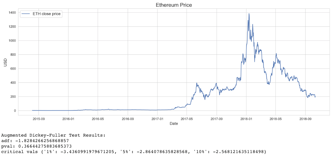
Looking at the ETH time series, it is clear that the mean close price near the beginning of the series will be much lower than at later points in time, particularly after around May 2017. This is to say, the series displays trend (or drift), which simply means that the data moves in a certain direction over time. More accurately, this series displays multiple trends, as there are periods of time where close price is trending upwards and others where it is trending downwards.

While obvious here, it is a good practice to follow up conclusions made from visual inspection with a formal test where applicable. Here, I am using the Augmented Dickey-Fuller (ADF) test, which is a null hypothesis significance test (NHST) for which the null hypothesis is that the time series has a unit root (trend), and the alternative hypothesis is that the series is stationary. The results shown here are the test statistic, p-value, and critical values from the output of the Statsmodels ADF test implementation in Python. Interpreting ADF results is simple: for significant values of p, the more negative the adf statistic, the stronger the rejection of the null hypothesis that a unit root is present. Statsmodels also outputs the critical values for the adf statistic at 1%, 5%, and 10% intervals. Simply put, critical values are points used to compare the test statistic with in order to determine whether to reject the null hypothesis or not. Here we don’t need to go beyond the p-value, as for a significance of p = 0.05, the value of p = 0.366 means we cannot reject the null hypothesis that there is a unit root present. As suspected, the series is not stationary.

Stabilizing ETH time series with differencing

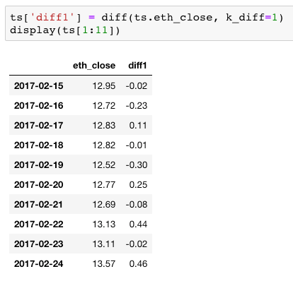
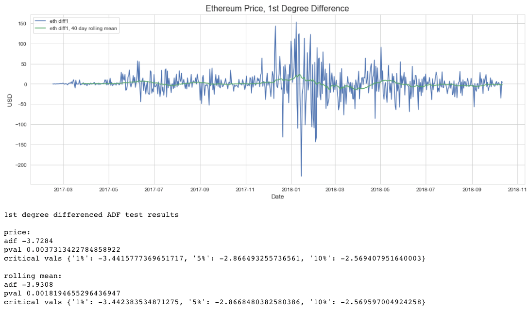
As stationarity is a common assumption underlying many time series analysis and modeling techniques, it is necessary to stabilize the data to achieve a stationary series. Differencing is an extremely common technique, and just involves computing the differences between observations. First degree differencing is the difference between consecutive values, and while often sufficient to stabilize data (as is the case here), it may be necessary to take the difference more than once or employ other techniques (such as square root, log, or log differencing). Here are the results of first degree differencing:

Interpreting these ADF test results for price, and keeping in mind a significance threshold of p = 0.05, the p-value of 0.0037 means we can compare adf = -3.7284 to the critical values. Since 3.7284 is less than the 1% critical value -3.4424, we reject the null hypothesis that a unit root is present and have a stationary process to work with.

What is this rolling mean business?

This visualization also includes a plot and ADF test for a 40 day rolling mean. The rolling mean is simply the mean of a moving 40 day window throughout the series, i.e. starting at index 0, it is the mean for observations 0 to 40, 1 to 41, 2 to 42, and so on until the end of the series. Why this is included (and why I am taking 40 observations at a time) will be covered in part 3 of this analysis, which will discuss structural breaks, change point detection, and rolling window forecasting.