Ethereum Time Series EDA Pt. 3

In-sample vs. out-of-sample forecasting

In time series, in-sample and out-of-sample forecasts are most easily explained in terms of train and validation/test sets. The approach is a familiar one - a model is fitted using a train set, then the model makes forecasts using test set feature data. A model is forecasting in-sample if it was fitted on the observation it is forecasting (i.e. included in the train set). Out-of-sample (OOS) forecasts are those made for observations that the model has never seen before (those contained in the test set).

When considering the end goal of predicting the time series’ future movements, it follows that a model’s out-of-sample forecasting error is the true measure of its predictive power. Of course, in-sample error remains important, as time series models can overfit just like any other.

Structural breaks and change point detection

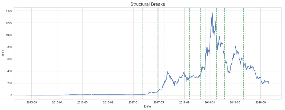
A structural break (sometimes called regime shift or change) is a sudden, unexpected shift in a time series’ behavior. Recall that a stochastic process is a sequence of random variables drawn from the same probability distribution. In statistical terms, a structural break occurs when a time series’ underlying probability distribution changes. Change point detection (or analysis) process which aims to identify when these changes or shifts happened, often by using an algorithm to compare statistical properties of the original and new distributions. While there are many approaches to change point detection, the two utilized in this analysis are given a quick look next.

Pruned Exact Linear Time (PELT)
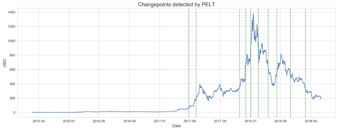
Introduced in 2012, PELT is a change point detection algorithm that works by minimizing a cost function over pruned segments of data. Segments are defined to start at t and end at T, and the change point in question is denoted s, such that t < s < T. The algorithm minimizes the summed cost of segments [t, s] and [s, T] with respect to the cost of the full segment [t, T].

Prophet
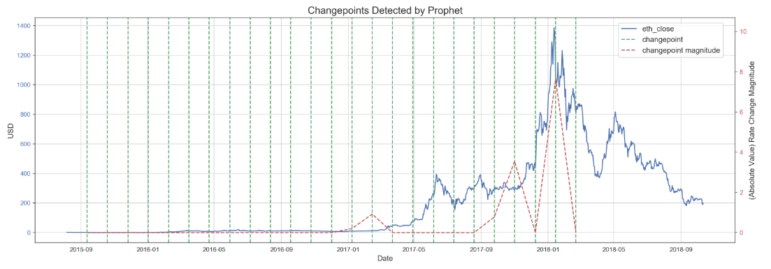
Prophet is an open source additive regression algorithm developed at Facebook. While best applied to data with seasonality (which is not a component here), I decided to use it’s built in change point detection to compare with change points detected by PELT.

As evident by the charted change points detected by each algorithm, PELT’s segmenting method ignores the beginning of the series, which Prophet detects. However, Prophet also contains a way to determine the magnitude of the change point, and after extracting Prophet’s significant change points (determined to be those with a greater magnitude than the mean of all change point magnitudes) and combining them with PELT’s change points, the following visual represents the final change points used for the rest of the analysis.

Recursive vs. rolling forecasts

Out-of-sample forecasts are typically done using either a recursive or a rolling forecast. Letting h denote the number of forecasts (or steps), a recursive (expanding window) forecast is done by fitting the model to the training data and producing h forecasts using test data. The training sample is then increased by one observation, the model is re-trained, and h forecasts are again produced.

Similarly, rolling (moving window) forecasts are performed by training the model and making h forecasts. However, the train set for the next iteration remains constant in size, but is moved ahead one time period. Where the expanding window retains the series history, the rolling window ‘forgets’ the oldest observation at each iteration.

At first, it may seem suboptimal to not train a predictive algorithm on all available data, but rolling forecasts offer a few distinct advantages over recursive ones. Thus, choosing a forecasting method requires consideration for the characteristics of the series that is being forecasted, as well as characteristics of the algorithms which will be producing the forecasts. While not an exhaustive list, the factors I assigned the most weight in choosing the method in this analysis are:

• Series length: the longer the series, the larger the train set will eventually become. This can result in significant computational costs when refitting to each train set, especially when using neural networks (which I use later in this project). Conversely, a rolling forecast results in relatively stable training times.
• Structural breaks: since a recursive forecast contains all past data, it is vulnerable to shifts in a series’ structure, whereas the rolling method’s “forgetfulness” offers some protection against these regime changes.

Window size

When using a rolling forecast, it is up to the user to choose the size (or length) of the window. A shorter window results in a smaller dataset for models to train with, risking suboptimal parameter estimation. However, a larger window may be long enough that it includes data from a previous regime. Recall that a shift in regime means that the underlying distribution has changed, and the process generating the data for a previous regime is no longer indicative of the current process. Thus, the larger window introduces the risk that the overall model itself may not capable of explaining variance for all included observations.

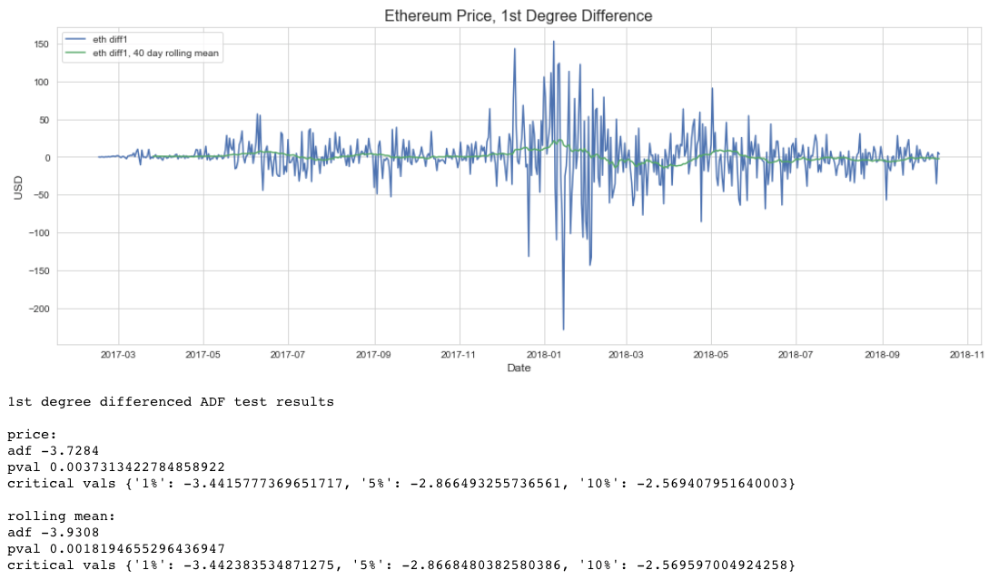
Thus, given the volatile nature of ETH price movements and multiple regime changes, I decided to use the median regime length as the window size. The intuition behind this choice was an attempt to maximize the data models trained on, while minimizing the amount of regime changes that a single training set would contain while iterating throughout the entire time series.

To back this up, I ran a window sized (40 observations) rolling mean ADF test to check that the series was stationary within this window size. As indicated below, the series is more stable within a 40 day interval than as a whole.

In the next post, I will introduce Auto Regressive Integrated Moving Average (ARIMA) modeling and discuss how it performed on this Ethereum time series.