ARMA and ARIMA: Preliminaries and Setup

AR and MA Models

ARMA and ARIMA models are best understood as combinations of their two core components: autoregressive (AR) and moving-average (MA) models.

Autoregressive models represent time-varying processes by calculating values for the target variable as linearly dependent on their own previous values, as well as a random noise term (often called a stochastic term). Autoregressive models use the notation AR(p), where p is the order (or number of autoregressive terms included). The AR term is thus written as:

Where c is a constant, are the parameters, and is the noise term.

Moving-average models essentially represent the error term as linearly dependent on its current and past values. Notated as MA(q) where q is the order (or number previous error terms included), the MA term is written:

Where is the expectation of , is the noise term, and are the parameters.

Time Series Regression: ARMA and ARIMA Models

ARMA (AutoRegressive Moving Average) models combine autoregressive and moving-average models into a single model. Given the above definitions of AR and MA polynomials, the ARMA model notated ARMA(p,q) is written:

To model a stationary stochastic process, an ARMA model uses the AR component to model the target variable, and the MA component to model the error. But as discussed in previous posts, not all stochastic processes are stationary. For these cases we have the ARIMA (AutoRegressive Integrated Moving Average) model, which is essentially an ARMA model with a built in differencing step for non-stationary processes. This differencing step is represented by the “integrated” part of the model, the order of which is assigned to d. Thus, if ARMA order is notated ARMA(p,q), it follows that ARIMA order is notated ARIMA(p,d,q). Functionally, the “integrated” aspect of the ARIMA model replaces values with those that have been differenced with d previous values.

Identifying Order: Autocorrelation and Partial Autocorrelation

When implementing an ARMA or ARIMA model, it is up to the user to set values for p, d, and q. One could simply try different combinations of AR and MA term orders, but a more methodical approach involves using ACF and PACF (AutoCorrelation and Partial AutoCorrelation Functions). Both ACF and PACF calculate coefficients of correlation between original and lagged versions of a time series, the difference being that PACF removes the effects of in-between lags. In practice, ACF is used to identify MA order q, whereas PACF’s characteristic of controlling for in-between lags make it useful for determining AR order p and I order d. (Note that d is often identified during the exploratory data analysis, as it is the same as the degree of differencing necessary to stabilize a non-stationary process. If d is already known, then simply use the stationary series to identify AR and MA order.)

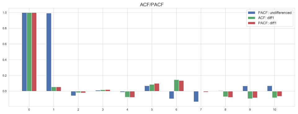
The number of lags plotted against ACF/PACF correlations (calculated using statsmodels) on the Ethereum time series is shown here:

To interpret these results, one compares the number of lags (x-axis) to its corresponding correlation (y-axis). In short, we are looking for positive correlations at lags before the correlation becomes negative and starts to fluctuate (which is just a result of noise or randomness).

At 0 lags, each function returns a perfect correlation of 1.0, as one would expect. This should be the case on any series, and including it in the ACF/PACF output is an easy check that the functions are running properly. This output is simply the function calculating the correlation between the value observed on day t and the value observed on day t lagged 0 times - itself. If this is not 1.0, something is wrong with the function’s implementation.

At 1 lag, there is a very strong (but not quite 1.0) partial autocorrelation on the undifferenced series. This indicates that d is at least one, and looking at the negative PACF value at 2 lags, we can comfortably determine that d = 1. Note that this is consistent with the first degree differencing used to achieve stationarity in EDA Pt. 2. Identifying d helps inform a couple of decision points. First, we know to use an ARIMA model rather than an ARMA model, as d = 1 making use the I term necessary. Second, we can use the stationary first degree differenced series to aid with AR and MA order determination.

Making sure to use a stationary series for inferring AR and MA term order, ACF and PACF calculate clear but weaker positive correlations at 1 lag, both of which become negative at 2 lags. Since p and q are integers, but the strength of the auto and partial autocorrelations are questionable, I built ARIMA models using AR(0), AR(1), MA(0), and MA(1) orders to compare. In the next post, I will implement and evaluate rolling out of sample forecast ARIMA models using the Ethereum time series data.